CS 452/652 Winter 2024 - Lecture 15

Train Modelling

Mar 5, 2024 prev next

Aside: think about stress-testing your kernel!

Train Modelling - Velocity

• Kinematics: area of Mechanics (and thus Physics)
• studies "motion of objects without reference to the forces which cause the motion."
• model trains emulate real trains
• we model the model trains
• velocity is inherently an average: distance / time

Goals / Objectives

• location tracking
  • collision avoidance
  • accurate stopping
• train efficiency: complete trips as fast as possible

Experiments and Data

• how many speed levels to investigate?
• determine minimum speed (per segment?) to avoid getting stuck
• stop from lower speed is more accurate
• how much data can you feasibly collect?
• document and justify decisions!

Measurement

• recommendation: use tight polling loop (no kernel)
• sensor → timestamp
• measurement errors
  • signal delivery, Märklin processing: constant (?)
    • constant errors cancel out when subtracting timestamps
  • delivery to software: variable (polling loop)
    • statistical modelling (see below)
  • processing in software: ignore small errors

Uncertainty

• assume actual sensor times uniformly distributed across duration of polling loop (~60ms)
• time interval between two sensors is sum of uniform distributions
  • general case: Irwin-Hall distribution
  • special case (N=2): triangular distribution
  • sample mean/variance are good estimates of real mean/variance
  • could also use min/max to estimated midpoint?
• but velocity (distance/time) is non-linear in time!
• average of time is straightforwarded; average of velocity not so much
  • consider simple example: 100m distance, 2 time samples 10s, 20s
  • speed: 10m/s, 5m/s → average would be 7.5m/s
  • compute average time first, then speed: 100m/15s = 6.66m/s
• observation: measured data typically forms bimodal distribution
  • why? is that a problem?
  • low-frequency sampling (60ms): sample distribution bimodal (corner cases trimodal)
• general recommendation: keep experiment raw data as much as possible
  • bug in processing → repeat only processing
  • new approach to data processing → possible with raw data

Dynamic/Continuous Calibration

• verify validity of and/or update current estimates
• long-term variability: track degradation? (or improvement)
• real-world variations (wear and tear): difficult to model
• need window of recent measurements
• basic technique: Exponentially Weighted Moving Average (EWMA)
  • c: current estimate; d: next data sample, α: weighting factor
  • c := c * (1 - α) + d * α
  • no need to store array of samples
  • with appropriate choice of α, can use bitshift instead of division
  • can use similar approximation for standard deviation

Train Modelling - Acceleration

• velocity is the derivate of movement
• acceleration is the derivative of velocity
• deceleration is negative acceleration
• kinematic reality:
  • velocity is finite → movement must be continuous
    • alternative would be teleportation
  • acceleration is finite → velocity must be continous
    • infinite forces would tear train apart
• simplified kinematic model: assume constant acceleration
  • approximate as average velocity during acceleration interval
  • or approximate as velocity step change in the middle of acceleration interval
  • both are ok, if somewhat lower-quality location estimate is acceptable during acceleration

Measurement

• measure similar to velocity
• measure time between two sensors
• change speed level at first sensor
• compute acceleration based on known estimates for velocities
  • first detect whether train has reached target velocity at 2nd sensor?
  • constant acceleration → average velocity during acceleration = (v₁ + v₂) / 2

Processing

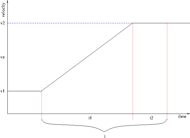
• assume acceleration from known velocity v₁ to v₂

  • experiment changes the speed at a sensor and measures the time to another sensor hit
  • measure times and estimate time averages first, as before!
  • t: average time; d: distance
  • average velocity during completed acceleration: v_a = (v₁ + v₂) / 2

• Scenario 1: acceleration complete before 2nd sensor hit (d/t > v_a)
  

  • split d into two segments d₁ (acceleration) and d₂ (stable velocity v₂): d = d₁ + d₂
  • split t into corresponding segments: t = t₁ + t₂
  • v_a = d₁ / t₁
  • v₂ = d₂ / t₂
  • can solve for d₁, d₂, t₁, t₂
  • acceleration: (v₂ - v₁) / t₁

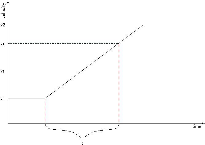
• Scenario 2: acceleration not complete before 2nd sensor hit (d/t < v_a)
  

  • actual average velocity during acceleration: v_s = d / t
  • velocity at 2nd sensor hit: v_r = v_s + (v_s - v₁)
  • acceleration: (v_r - v₁) / t

• if d/t = v_a, both methods work

Stop Distance

• special case of deceleration
• manual experiment
  • send stop command when sensor is triggered
  • manually measure stop distance

Stop Time

• compute using acceleration model
• experiment with two sensors close to each other?
• experiment by trying to stop right after sensor
  • use search algorithm to find right time: could be automated
  • stop time + velocity → compute stop distance?
  • search algorithm (e.g., binary search) might be brittle and need many experiments

Start

• special case of acceleration
• measure based on known estimate for stop time/distance
• stop at known location, then start
• measure time to sensor
• can compute acceleration
  • similar caveat as acceleration measurement: did train reach target velocity?

Short Moves

• stop before reaching target velocity
• manual experiments with different (short) times between start and stop

Earlier Documents

The material covered in class should be sufficient for train modelling. However, during the past years, various documents have described train modelling and calibration in the context of CS 452/652. The various versions are made available here with the caveat that they might or might not be helpful:

Stopping (2016)
The Kinematics of Train Calibration (2017)
The Kinematics of Train Calibration (2015)
Reverse Engineering Acceleration/Deceleration(2011)