M10: Binary Trees

In this video we’ll look at some introductory examples (including one not on the slides) and the definition of a tree.

Video: Download m11.10_intro

In some trees, each internal node will always have exactly two children while others may have an unlimited number. That’s a useful thing to know when writing the code! Similarly, it’s useful to know whether the order of the children matters or not.

We’ll be refering back to these characteristics for most of the trees that we discuss.

In the mean time, consider the binary expression tree. Each internal node has exactly two children. That’s implied by the “binary” in the name – it only deals with operators having a left and a right operand. If we added/allowed an unary minus then each internal node would have at most two children (because the unary minus would have only 1).

In Module 13 we’ll look at another kind of arithmetic expression tree that can have any number of children. It represents (+ 1 2 3 4) as a “plus” node that has four children.

The order of the children matters in a binary expression tree. If we swapped the children of the division operator, we would get a different result when evaluating the expression. The order of the children in the phylogenetic tree does not matter.

All of the trees we’ve looked at so far derive their structure from the data. That won’t be the case for a binary search tree (BST). In that case the structure will be very important to enable fast searching, but it will be a structure that we decide rather than one that comes from the data itself.

Binary trees are about as simple as trees get. Characteristics:

• Each internal node has at most two children.
• Our examples will have labels on all the nodes, although that’s not a requirement of binary trees.
• Order of the children does not matter.
• Structure is for convenience.

Work through the next five slides. The last one is deliberately incomplete. Attempt to complete the template on your own. Then watch the video to check your process and the result.

The BT data definition is an example of mixed data. One case is a particular kind of list, an empty list. The other case is a structure. We can use the type predicates empty? and node? to distinguish them.

We could have used many other values instead of empty – any value that we can distinguish from a Node. We could have used 0 or false or 'empty-tree. We chose empty simply because its an existing value that strongly suggests “empty tree”. The fact that empty has significance for lists is not relevant here.

The following video works through building bt-template based on the data definition.

Video: Download m11.20_bt_template

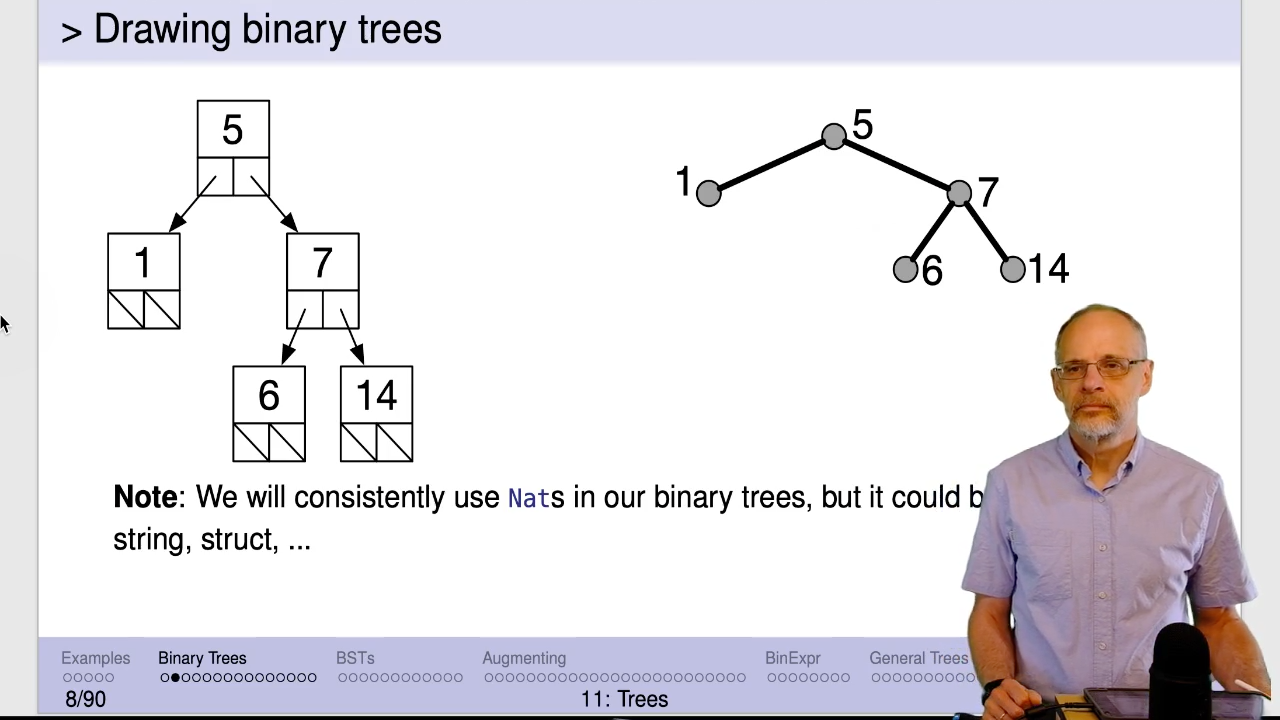
It’s worth taking a look at the check-expects to see how a tree is built. Use the structure constructor make-node and provide it with three values: the key at the root of this (sub)tree, the left subtree and the right subtree.

The subtrees may be empty or they may be a non-empty subtree constructed with (you guessed it!), make-node.

Take a look at the Key Questions on the next slide; then come back and try implementing sum-keys. Use the template!

Video: Download m11.30_sum_keys

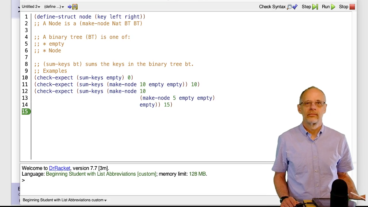
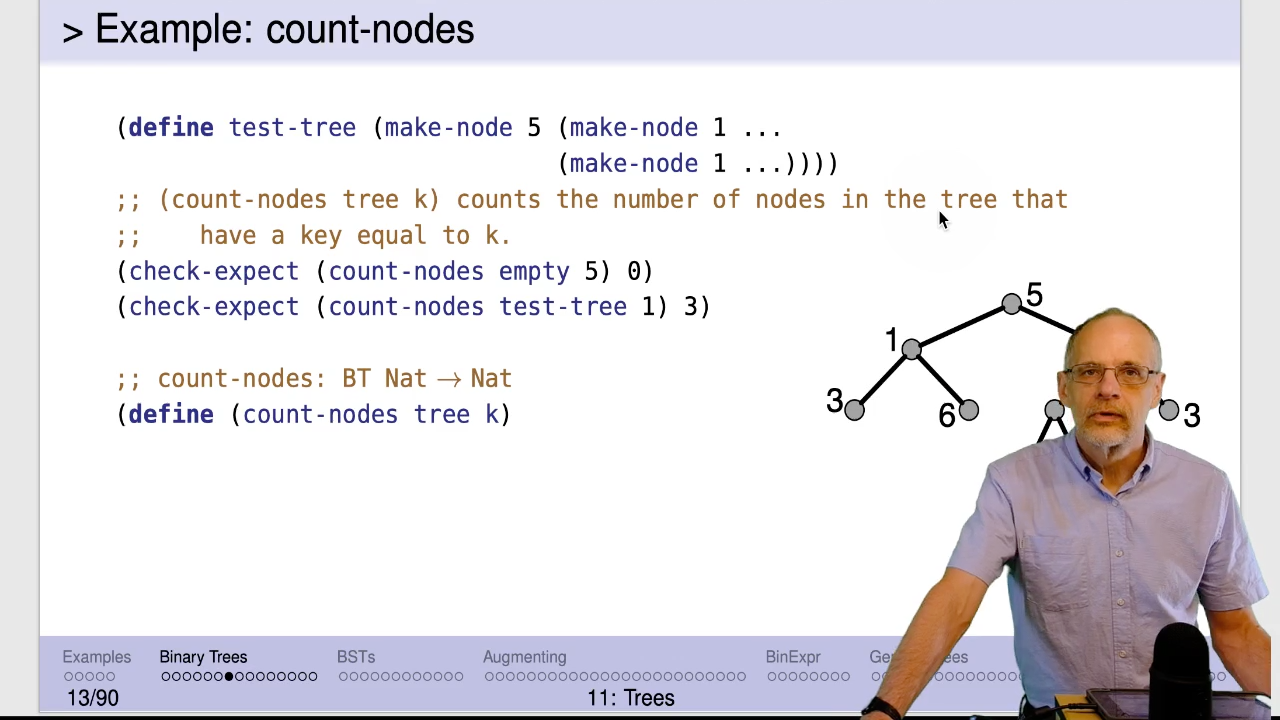
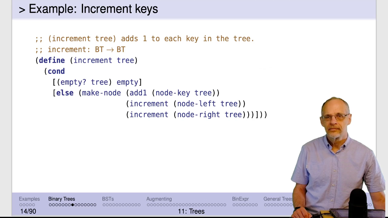
Note the similarity to the template for sum_keys, count-nodes, and increment (next slide). That’s no accident!

It’s important to break tree problems like these into recursive subproblems. Each of these three short videos talks about the strategy for doing that.

Video: Download m11.35_count_nodes

contains? might be a better name for search-bt. It is a predicate, after all, and the question mark in contains? follows our convention for predicates.

Since it produces a Boolean, we might think about whether we can write this as a Boolean expression, without the cond.

In the example tree shown, the result of (search-bt-path 9 t) (where t is the tree shown) is (list 'right 'right 'left). Why? Put your finger on the root node. The first item on the list is 'right. So move your finger to the root of the right subtree (10). The second item on that list is also 'right. Move your finger to the root of the right subtree (7). Do it one more time, moving left this time, and you arrive at 9.
Your finger has traced a path in the tree from the root to 9.

What’s the path to 6? Start with what’s given: the path from 6 to 9. Based on that, it seems reasonable that (list 'right 'right) would be the path from 6 to 8 and just (list 'right) is the path from 6 to 10. Making the path one element shorter, (list ) or empty gives the path from 6 to 6.

This is shown in the second check-expect on the next slide.

Take a careful look at the contract. Does it make sense to you?

What’s the strategy for solving this problem?

Well, a non-empty tree has three important parts: the root, the left subtree and the right subtree.

If the root contains k, the value we’re searching for, produce empty and we’re done.

Otherwise, if only we could find a path to k in the left subtree, we could cons 'left onto that path and we’d have the answer from the root.

If we can’t find k in the left subtree, we could look in the right subtree. If we can find a path there, all we need to do is cons the value 'right on to that path and we’d have the path from the root to k.

If k isn’t in the root, isn’t in the left subtree, and isn’t in the right subtree, then it’s not in the tree at all and we should produce false.

How do we check if k is in the left subtree? Apply search-bt-path. If it produces a list, we know k was found. We could also check for the result to be not false.

However, after we’ve checked if k is in the left subtree we still need to have the path to k so we can produce (cons 'left path-to-k). To get the path to k we need to call search-bt-path a second time.

This strategy leads to the code shown on the slide.

The code is correct and works as intended. However, that second application leads to incredibly inefficient run-time, as we saw in max-list . We’ll fix that in a moment.

Before we do that fix, note that this code doesn’t look that much like the binary tree template:

;; bt-template: BT -> Any
(define (bt-template t)
  (cond [(empty? t) ...]
        [(node? t) (... (node-key t)
                        (bt-template (node-left t))
                        (bt-template (node-right t)))]))

There are some points of similarity:

• Both check for the empty tree as the first clause in the cond.
• Both apply themselves recursively to both the left and right subtrees.
• Both do something with the key at the root.
• The last four clauses of the cond could have been nested inside the 2nd clause of the template, making it look more similar.

The next version of search-bt-path actually looks much more like the template while also solving that efficiency issue.

We solved max-list three different ways:

• The very, very slow version which applied max-list recursively multiple times for each recursive application.
• Using a helper function, max (which happens to be built-in).
• Using an accumulator.

We could use either a helper function or an accumulator to solve this efficiency problem, too. The helper function approach is simpler and is the approach pursued here.

The insight is that once a value is passed to a parameter it can be used multiple times without recalculating it. So we search for k in both the left and right subtrees, passing the results to the helper function. choose-path can use those values multiple times without incurring the efficiency penalty.

One might object that this always searches the entire tree. In particular, the right subtree is always searched even if k has already been found in the left subtree. Isn’t that wasteful? Yes. But not nearly as wasteful as those double applications we got rid of. We could improve this further, but it would be a pain. Besides, we’ll see better approaches in module 14.

So how many different BSTs for n keys are there?

• 0 keys, there is exactly 1 binary search tree (the empty tree).
• 1 key, there is exactly 1 binary search tree.
• 2 keys, there are two possible binary search trees (draw them!).
• 3 keys, there are five possible binary search trees (draw them!).

For 4 keys, k₀ < k₁ < k₂ < k₃:

• If k₀ is the root, there are 0 keys in the left subtree and 3 keys in the right subtree. So there are 1 x 5 = 5 possible trees with k₀ at the root. Why?
  The 0 keys in the left subtree can be arranged only 1 way (an empty tree). But the three keys in the right subtree can be arranged five different ways (see above).
• If k₁ is at the root, there is 1 key in the left subtree and 2 keys in the right subtree resulting in 1 x 2 = 2 possible trees.
• If k₂ is at the root, there are 2 keys in the left subtree and 1 key in the right subtree resulting in 2 x 1 = 2 possible trees.
• If k₃ is at the root, there are 3 keys in the left subtree and 0 keys in the right subtree resulting in 5 x 1 = 5 possible trees.

Summing these possibilities, we get 5 + 2 + 2 + 5 = 14 possible BSTs with four keys.

The last clause, (> n (node-key t)), could be replaced with else.

Remember the increment function we examined earlier? It consumed a tree, t, and produced a transformed tree, t'. This is doing essentially the same thing and will use the same techniques.

What’s the contract for bst-add? It consumes a new key and a BST. It produces a BST, so the contract is bst-add: Nat BST -> BST.

In each of these cases we produce a BST, either empty or a Node.

When we consume a node that does not match the key, we need to produce a new node containing the old key, the transformed subtree, and the untransformed other subtree.

All of these functions should make use of the BST ordering property to save work.

Refer back to the code for search-bst and note how little has changed:

• Add val to the node structure.
• If (= k (node-key t)) is true, produce (node-val t) instead of true.
• The purpose and contract.

Binary expression trees were one of the motivating examples at the beginning of this module. To briefly recap, a binary expression tree structures arithmetic expressions into a tree which makes it easy to calculate the value of the expression.

This core idea is used in programs that consume an expression from a user and then calculates the value. It’s also used in compilers and interpreters that consume source code (like your Racket programs!) and execute them.

What’s in the name “Binary arithmetic expression tree”? Let’s start at the back:

• Tree: we’re organizing information into a tree structure
• Arithmetic Expression: The information we’re organizing are “arithmetic expressions” – expressions that represent arithmetic, like 5 + 2. There are other kinds of expressions. For example, we could represent Racket cond expressions in a tree. But we’re not trying to handle them at this time.
• Binary: We’re not even trying to handle all arithmetic expressions, only those that have two operands. So functions like square root or cosine are out. So is the unary minus operator. In our example, we’ll focus on the classic four: +, -, *, /.

The slide refers back to the tree characteristics we commonly care about.

The smallest possible binary arithmetic expression tree is a single number (the first example). The next smallest tree is two numbers and an operator (see the second example). A binary arithmetic expression tree can grow to be arbitrarily large.

Leaf nodes in a BinExp will always be numbers. Internal nodes will always have an operator with left and right subtrees that are binary arithmetic expressions.

The last tree represents our running example, the expression (2 * 6 + 5 * 2) / (5-3).

Calculating the value of this BinExp is simple: calculate the value of the left subtree, calculate the value of the right subtree, and then divide.

When the subtree is just a number, it’s value is that number.

When an expression is represented as a tree, it automatically encodes the precedence rules. For example, our usual rules interprets 1 + 2 * 3 as 1 + (2 * 3) or 7. That corresponds to an expression tree with + at the root and 2 * 3 in the right subtree.

If we wanted the other interpretation, (1 + 2) * 3, the expression tree would have the * at the root and 1 + 2 in the left subtree. Either way, the tree eliminates the need for the parentheses or special rules.

The templates follow naturally from the data definitions. In this case we’ve done the full template – a template for a BINode and a template for a BinExp.

Let’s turn now to actually evaluating a binary expression.

The eval function consumes a BinExp and produces its value (a number). The binexp-template consumes a BinExp, so start with it. It distinguishes between a binary expression that is just a number and one that’s more complicated. In the first case, that number is the answer; just return it. In the second case, we have a BINode, so write a helper function based on binode-template.

For each of the four arithmetic operators, we check which one it is, calculate the values of the left and right subtrees and then do the right thing for that operator using the built-in function.

Note that the left and right subtrees may be either a number (a leaf node) or a subexpression (a BINode). eval can handle either one of those whereas eval-binode can only handle a BINode; so eval is the right function to apply.

Unfortunately, there is a lot of repeated code in eval-binode on the previous slide:

• We evaluate the left subtree at four different places.
• We evaluate the right subtree at four different places.
• We extract the operator from the binode structure at four different places.

The code on this slide pulls those three operations into eval and passes the results to eval-binode instead of the subtree itself. The result is much cleaner code without the repetition.

What happens if the binary arithmetic expression tree contains a modulus operation? Nothing evaluates to true in eval-binode’s cond expression, generating an error. It would also be easy to implement the modulus operator, but then what about exponentiation? It might be wise to add an else (error "Unimplemented operator") to make debugging this kind of error easier. Try it!

In Module 14 we’ll be able to take this one step farther and even eliminate testing which symbol we have in the expression tree. What’s the secret? We’ll store the function itself in the tree instead of a symbol. It’ll be fun!