M13: Local Definitions

Change DrRacket’s language level to “Intermediate Student”. Keep the other settings as described in M02-009 .

“Arbitrarily nested” means expressions can have subexpressions, conds inside conds, lists can be nested within lists, lists can be inside structures (and visa versa), etc.

But that’s not true of define and check-expect.

We’re about to fix that for define. On the other hand, check-expect will always be required to be at the top level. “At the top level” simply means that it is outside of everything else; it’s not nested.

This slide and the next several present a computation that seems like it should be easy, but every way we express it has some objection. Those objections are mostly of the form:

• There’s too much repeated code!
• But this doesn’t look like the formula we’re implementing!
• The computations are separated and thus hard to understand!

Professional programmers try to follow the “DRY Principle”. DRY stands for “Don’t Repeat Yourself”.

Repeating yourself:

• Allows bugs to be fixed some places but not others.
• Is often less efficient for the computer.
• Involves more typing for the programmer.
• Means the code must be understood again each time it occurs.

According to Wikipedia , violating the DRY principle results in a WET solution. WET is commonly understood to stand for “Write Every Time”, “Write Everything Twice”, “We Enjoy Typing”, or “Waste Everyone’s Time”.

Here the DRY violation is particularly obvious but not particularly egregious because the code is so simple and concentrated in one place. But it points towards a general problem that needs to be solved.

Obviously, local will be one technique to help “DRY things up”. The other major technique you already have in your toolbelt: helper functions. In M16, we’ll introduce another technique, higher order functions.

This approach is just plain silly. There is no advantage and several disadvantages.

Here, the helper function calculates the value of s in the original formula.

Note that it’s called four times. This calculation is “cheap” to compute, but many others are not and repeating them four times could have a significant impact on the speed of the program.

The helper function also has a terrible name. But what should you call it? It has no meaning outside of the calculation of Heron’s formula. So name it calc-s-for-herons-formula? Yuck!

In addition to being more readable and shorter, this solves the DRY problem. The code to compute s is not repeated. It doesn’t have to be typed multiple times and it doesn’t have to be executed multiple times.

But we’d like to keep related code together, if at all possible.

Now, you might be thinking, “t-area-v3 is just a wrapper function; we’ve done that lots of times and no one has complained.” Uh huh. Now we’re complaining. Because now we have the means to fix that.

Finally! Advantages of this code:

• It’s DRY. Nothing is repeated.
• Calculations are only performed once.
• It keeps everything related to calculating Heron’s formula together in a single function.
• Because the definition of s is so contained, we don’t need to give as much thought to naming it.

This code calculates the value of (/ (+ a b c) 2) and binds it to the identifier s. That value is then used in place of s everywhere in the expression (sqrt (* s (- s a) (- s b) (- s c))).

What do we mean by “permit reuse of names”? In the code on the slide, programmers have better things to do than worry about whether a parameter name (n) conflicts with a constant name (also n). So the designers of Racket (and other languages) defined the rules to make it easy. Names can be reused. In broad strokes, the closest definition “wins”.

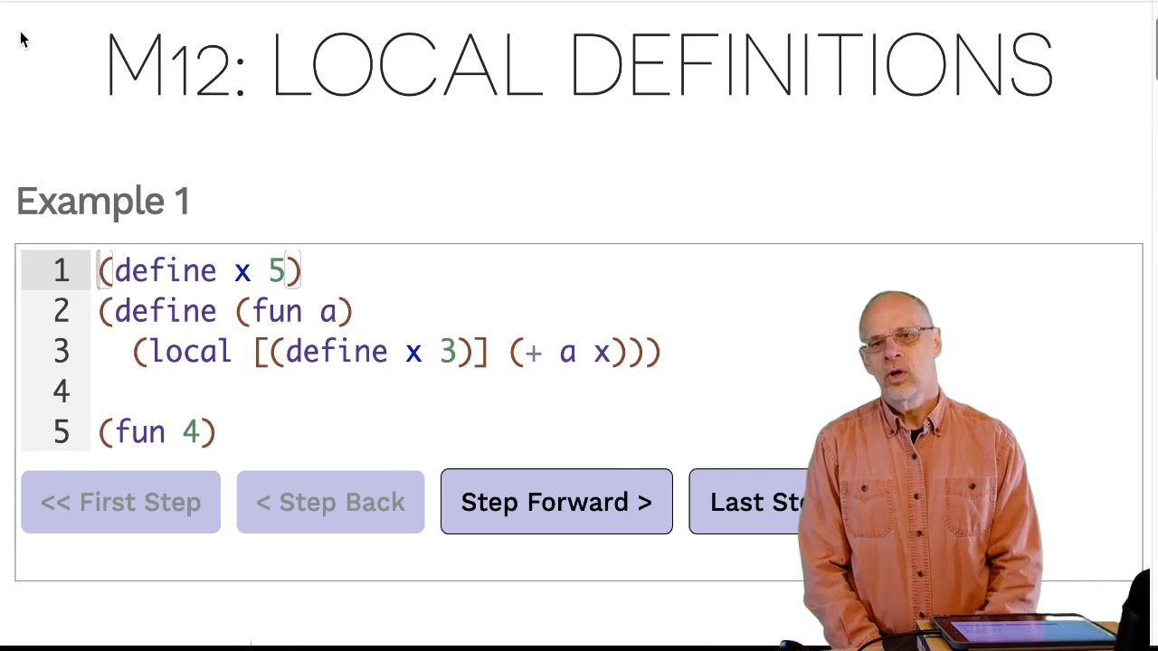
This same principle is extended to local. The following produces (+ 4 3), not (+ 4 5).

(define x 5)
(define (fun a)
  (local [(define x 3)]
    (+ a x)))

(fun 4)

Our substitution rules will need to handle these kinds of cases.

Example 1

Video: Download m14.10_semantics

1. Prepare to apply the user-defined function substitution rule.
2. Replace (fun 4) with the body of fun and 4 substituted for the parameter a.
3. Prepare to apply the local substitution rule.
4. Apply the local substitution rule. There are several sub-steps that are all done together:
   1. Come up with a brand new (“fresh”) name for the local definition of x that has not been used for anything else in this program. The stepper uses the name x_1. Use that fresh name, x_1, wherever the local definition of x was used (e.g. in (+ a x)).
   2. Move the definition of x (now called x_1) up to the top level of the program.
   3. Replace what’s left, (local [] (+ a x_1)), with just the local’s body expression, (+ a x_1).
5. Proceed to evaluate the program using the rules we learned before.

It doesn’t matter what the fresh name is, just so long as it hasn’t been used anywhere else in the program (that is, it really is “fresh”). It could be zorgon_59 or j$%#222. Racket will choose it and we’ll never know what it chose.

But in our stepping exercises, we’ll simply use the variable name followed by an _1. If we have a second identifier with the same name, we’ll use _2 and so on. We’ll assume that our programs won’t have both an x and an x_1, although Racket must handle that case.

Example 2

Video: Download m14.21_semantics

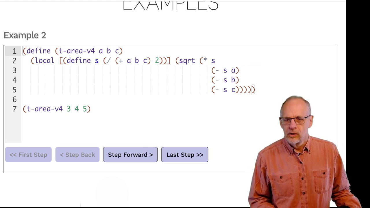
This example introduces a couple of new wrinkles:

• There are multiple parameters to substitute (but that’s not part of the local substitution rule).
• The local definition, s, is used multiple times. So s_1 will also appear multiple times.
• The definition of s involves a computation. It will be performed after the definition is moved to the top level, using the same rules as before.

Example 3

Video: Download m14.30_semantics

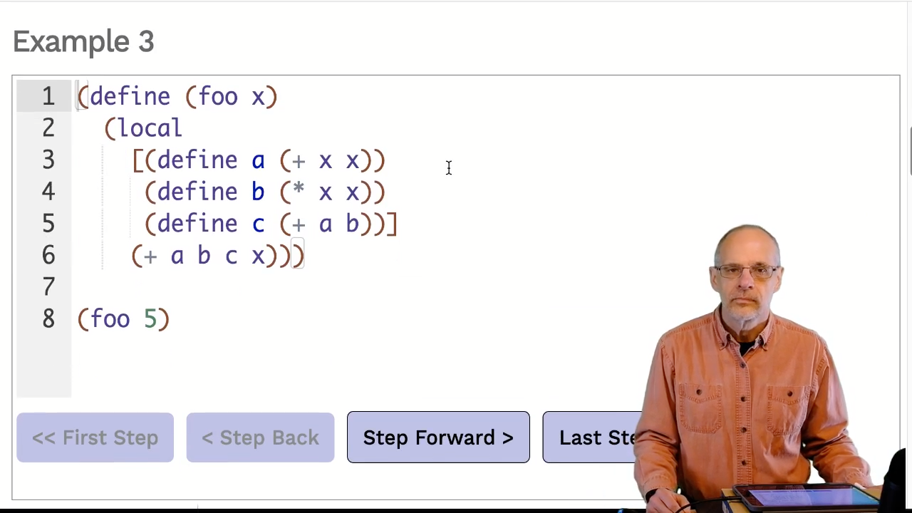
A local expression can have multiple definitions. They are all handled together as a single step.

The formal rule uses a pattern ellipsis (...) and subscripts to indicate an arbitrary number of local definitions.

Example 4

Video: Download m14.40_semantics

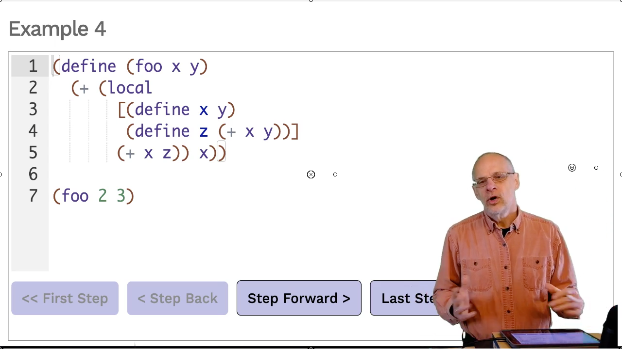
A local definition can be nested in an expression, as seen in this example. It doesn’t need to be at the top level of the define. Here, it will calculate a value that is then added to x. In the video we show a similar example where the local is nested inside the else for a conditional expression.

As you step through the example, pay particular attention to where x, the function parameter, is substituted and where x, the local definition, is substituted. Within the local, the (define x y) takes precedence over the parameter. Otherwise, the parameter is used.

Most programmers prefer to avoid having a local definition that “shadows” a parameter name. Why make things more complicated than they need to be? But it happens and so the rules need to handle it (and you need to know the rules).

Example 5

Video: Download m14.50_semantics

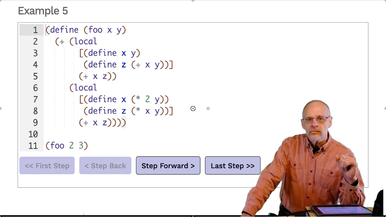
You may be wondering about all the fuss of a new, fresh identifier. The following example shows why it’s needed.

We have two local expressions within foo. Both define an x and a z that will be lifted out to the top level. If we didn’t have fresh identifiers for each of them, there would be a conflict.

The first x to be renamed and lifted will be x_1. The second will be x_2.

We’re now going to move more carefully through four reasons to use local. Some of these recall arguments made during the motivational example at the beginning of the module; “encapsulation” is new.

This is the second of the four reasons for using local. The four reasons are:

• Clarity: Naming subexpressions
• Efficiency: Avoid recomputation
• Encapsulation: Hiding stuff
• Scope: Reusing parameters

Refer back to Module 09 if you need a refresher on the problems encountered with max-list.

max-list-v2, repeated from M09.

In max-list-v4 we calculate the maximum of the rest of the list in the recursive case. Once that value has been calculated, the local allows us to use it multiple times without recalculation. Recall that it was recalculation that caused the efficiency issues with max-list-v2.

This is the fourth approach we’ve seen to finding the maximum value in a non-empty list:

1. max-list-v1 used the built-in helper function, max.
2. max-list-v2 had two recursive applications that led to significant efficiency issues.
3. max-list-v3 solved the problem with an accumulator.
4. max-list-v4 solves the problem with local.

Of the four, the first one is likely the best approach. Thanks to the built-in helper function max it’s a simple and direct approach that is also efficient. If max was not available, then either version 3 or version 4 would likely be considered the best choice.

This version of search-bt-path from Module 11, slide 18 suffers from the same problem as max-list-v2: it often applies itself twice to the same argument resulting in an explosive growth in the number of applications as the tree becomes larger.

This version uses local to avoid recomputing values.

The left-path is only computed if the outer else clause is reached. The path is checked and, only if required, is a second local evaluated and the right-path is computed.

Note that this is not the else (cond pattern from Module 03, Slide 26 . There is a local in between.

This is the third of the four reasons for using local. The four reasons are:

• Clarity: Naming subexpressions
• Efficiency: Avoid recomputation
• Encapsulation: Hiding stuff
• Scope: Reusing parameters

local also allows functions to be defined. When the local is evaluated, the function will be renamed with a fresh identifier and lifted to the top level of the program. For example,

We say the local function is “invisible” because it can’t be used outside of the local. For example, trying to run the following program

(define (gus x)
  (local [(define (foo x) (+ x x))]
    (* (foo x) (foo (+ x 1)))))

(gus 2)
(foo 2)

results in an error: foo: this function is not defined.

That means foo can’t be misused by applying it in an unintended context (outside of gus). It also means that foo can be removed from the list of functions most programmers need to worry about (that is, decluttering the top-level namespace).

local is often used with wrapper functions. The wrapped function – the one that does most of the work – is defined within the local.

This exercise is a bit more work than most of our exercises. However, once we introduce higher order functions in M16, this problem can be solved using local in only four lines of code! Without the techniques of M16 (and using local) it takes about 9 or 10 lines of code.

Here’s another example of code we’ve seen before rewritten with a local.

Note that insert is only required to have a purpose statement and a contract. Tests are not required (largely because check-expect can’t be nested).

is-even? and is-odd? are each given fresh names and lifted to the program’s top level. They then act just like any other pair of mutually recursive functions.

This is the last of the four reasons for using local. The four reasons are:

• Clarity: Naming subexpressions
• Efficiency: Avoid recomputation
• Encapsulation: Hiding stuff
• Scope: Reusing parameters

countup-to-v1 is similar to code from M07 where we need a helper function with two parameters – one for where we are counting from and the other to be our ending point. But the ending point, to, never changes. We’ve described that as “going along for the ride”.

Note how countup-from has the value of n (3) embedded in it when it is lifted out to the top level. Handy!

Video: Download m14.70_embedded_values

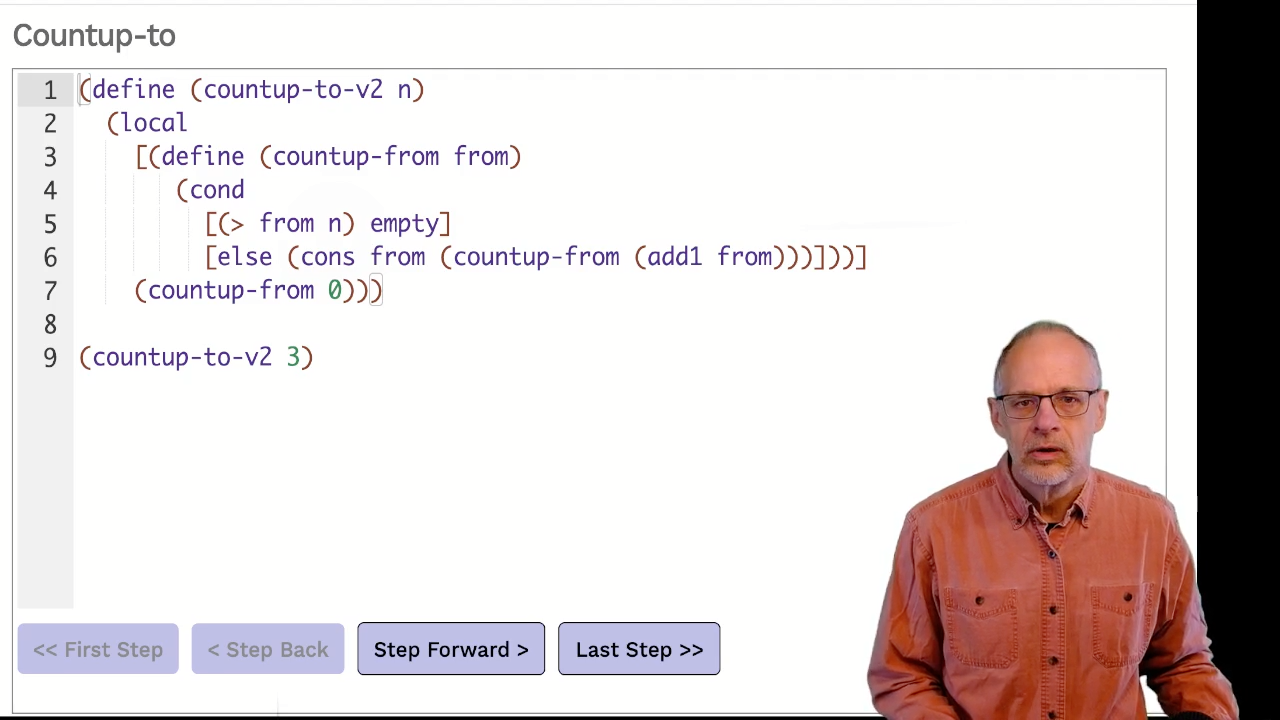
There’s no need to trace this for more than a couple of steps. Once the function is lifted out, you’ve seen what you need to see.

(countup-to-v2 10) and (countup-to-v2 20) both result in local functions being lifted to the top level. You may be wondering what happens to them after they have been evaluated and are no longer needed. There are two parts to the answer.

First, the substitution model is not necessarily the way the computation is actually implemented in DrRacket. It may have a more efficient way to do it.

Second, unneeded resources (including cons cells and lifted functions) are reclaimed in a process called “garbage collection”.

This is our second implementation of mult-table. The first was in M08 . The third (and last!) will come in M16.

There are a lot of values just going along for the ride in this code:

• In rows-to, both nr and nc (the number of rows and number of columns) are going for the ride; they never change.
• In cols-to, nc is going along for the ride.

By making rows-to and cols-to local to mult-table, the parameters nr and nc will be in scope and don’t need to be passed as parameters.

As with countup-to-v2 and its helper method, when the functions rows-to and cols-to are lifted to the top level they will have the values for nr and nc “embedded” in the body of the function.

Advantages to this version of mult-table include:

• Making clear that rows-to and cols-to belong to mult-table and are not expected to have other uses.
• Not needing to expend effort to determine that nc and nr really don’t change as the helper functions execute.
• Simplifying the parameters for the helper functions and thus reducing the chances that they are mixed up.

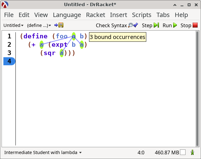
DrRacket can help you with these. If you click “Check Syntax” and then hover your mouse over a binding occurrence, it will draw arrows to the bound occurrences.

Hovering over a bound occurence will draw an arrow from the binding occurrence and highlight the other bound occurences.

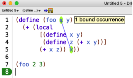
For an example of the “holes” mentioned in the definition of “lexical scope”, consider Example 4 from our earlier discussion:

The “holes” are the occurrences of x that are not highlighted due to (define x y).

When we first discussed the semantics of local we had not yet seen locally defined functions. This rule takes them into account.

The substitution rule uses indices like _1 to number the definitions in the local. Indices are used again to for the identifier in each definition (e.g. x_i). Unfortunately, we’ve ALSO been using indices to indicate the “fresh” identifiers in our past examples. Here, the fresh identifier is indicated by tacking on _new. That’s confusing! Sorry, but we ran out of notational ideas. If you’ve got a better idea of how to notate this, please let us know!